🔹 What is PVT Motion?

PVT Motion is another Streaming Motion. PVT Motion is a bit more complicated to use because it requires an array of Positions, Velocities, and Time deltas. The controller is only responsible for figuring out the acceleration for each motion segment. This makes it more flexible and gives users more control over the motion path.

It is important to note that the velocity argument specifies the target velocity of the axis at the given time, not how it moves between points. The average velocity between points is determined only by the difference in position and time. At the extreme, when the time deltas are a single sample, there is no room for interpolation, and the motion becomes equivalent to PT (the velocity input is effectively ignored).

Move PVT

Output Motion Scope

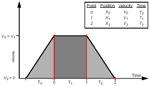
The PVT algorithm is very good for smooth and close path control. The points can be spaced very close or very far apart. For complex paths (or path portions) the points should be spaced close together. For simple paths (or path portions) the points can be spaced far apart. PVT can handle virtually any list of points. The most difficult part is determining the appropriate velocities at each point.

Trapezoidal move example:

pos[0] = 050; v[0] = 100; t[0] = 1;

pos[1] = 400; v[1] = 100; t[1] = 3.5;

pos[2] = 450; v[2] = 000; t[2] = 1;

Note: Both the Position and Velocity arrays are direction sensitive meaning you must put a (-) sign on negative numbers.

🔹 MultiAxis PVT Motion

All motion streaming methods can be used for coordinated motion on multi-axis objects. It is important that you set up your arrays appropriately for a multi-axis object. See the examples below on how to structure your arrays for multi-axis motion.

🔹 PVT Algorithm

A trapezoidal velocity profile motion could be generated using a list of three Position, Velocity, and Time points:

PVT profile (trapezoidal)

Calculate the change in distance between two points divided by the time:

This is a simple method with relatively smooth performance. You will need to add an extra final point to the list, setting the last velocity to zero.
Calculate a constant acceleration fit between points. From the kinematic equations (with Jerk = 0), we know:

Substitute (b) into (a) and solve for Vn+1:

There are several other methods that can be used to calculate the velocities. Additionally, there are many other algorithms, such as averaging and splines, that can be applied to PVT.

What happens if the Velocities are calculated improperly for PVT paths?

The PVT algorithm doesn’t care if the Position, Velocity, Time points are matched properly. The PVT algorithm will simply calculate a Jerk profile between points to reach the specified point. The profile between the points may not be desired, but it will be accurate.

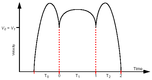
For example, consider the simple three point trapezoidal profile from the PVT profile (trapezoidal) graph above. If the velocities at points 0 and 1 were too small, the profile would stretch to cover the proper distance (area under the curve):

PVT profile, velocities too low)

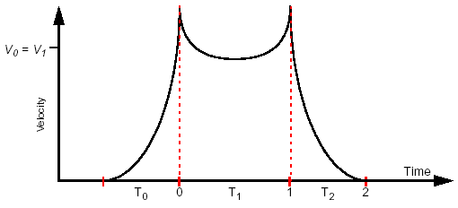
If the velocities at points 0 and 1 were too big, the profile would shrink to cover the proper distance (area under the curve):

PVT profile, velocities too high)

When is the PVT algorithm useful?

The PVT algorithm is very good for smooth and close path control. The points can be spaced very close or very far apart. For complex paths (or path portions) the points should be spaced close together. For simple paths (or path portions) the points can be spaced far apart. PVT can handle virtually any list of points. The most difficult part is determining the appropriate velocities at each point.

EXAMPLE 1 - Two-Axis MultiAxisXY with MovePVT

The position and velocity data for both axes are combined into the arrays. The time array is shared for both axes. This is why you need twice as many position and velocity points than you need time points. See the example below:

p[0] = 050; v[0] = 100; t[0] = 1;
p[1] = 025; v[1] = 050;
p[2] = 400; v[2] = 100; t[1] = 3.5;
p[3] = 200; v[3] = 050;
p[4] = 450; v[4] = 000; t[2] = 1;
p[5] = 225; v[5] = 000;

1st Segment

2nd Segment

3rd Segment

Resulting Motion Plot

AxisX

p[0] = 050;

v[0] = 100;

t[0] = 1;

p[2] = 400;

v[2] = 100;

t[1] = 3.5;

p[4] = 450;

v[4] = 000;

t[2] = 1;

AxisY

p[1] = 025;

v[1] = 050;

t[0] = 1;

p[3] = 200;

v[3] = 050;

t[1] = 3.5;

p[5] = 225;

v[5] = 000;

t[2] = 1;

🔹 PVT Motion with Feedforward (PVTF)

MovePVTF extends PVT motion by adding a feedforward term to each point. The feedforward value is a raw control output value applied directly to the control output, combining the smooth velocity-controlled motion of PVT with direct feedforward control.

When to Use PVTF

PVTF is useful when you need both velocity control and feedforward compensation:

High-Speed Coordinated Motion: Apply gravity or friction compensation during complex multi-axis paths
Model-Based Control with Velocity Constraints: Use calculated feedforward while maintaining specific velocities
Dynamic Load Compensation: Provide torque feedforward for robotic arms or systems with varying loads
Precision Contouring: Combine smooth PVT profiles with feedforward for improved tracking accuracy

Feedforward Units and Configuration

Feedforward values are raw control output values, not UserUnits:

Typically 16-bit signed integers for torque control (-32768 to 32767)
Typically 32-bit signed integers for velocity or position control
The axis must be configured separately for the output type and PDO mapping via demand channel configuration

Feedforward Interpolation

The feedforward values are linearly interpolated between consecutive points during multi-sample segments:

If a segment spans 10 firmware samples, the feedforward transitions smoothly by 10% per sample from the current point to the next
For single-sample segments, the feedforward changes instantly at each point

Array Structure for PVTF

For single Axis:

positions[]    = [p₀, p₁, p₂, ..., pₙ]
velocities[]   = [v₀, v₁, v₂, ..., vₙ]
times[]        = [t₀, t₁, t₂, ..., tₙ]
feedforwards[] = [f₀, f₁, f₂, ..., fₙ]  // raw control output values

For MultiAxis with 2 axes:

positions[]    = [X₀, Y₀, X₁, Y₁, ..., Xₙ, Yₙ]
velocities[]   = [Xv₀, Yv₀, Xv₁, Yv₁, ..., Xvₙ, Yvₙ]
times[]        = [t₀, t₁, ..., tₙ]
feedforwards[] = [Xf₀, Yf₀, Xf₁, Yf₁, ..., Xfₙ, Yfₙ]

Note: The feedforwards array size must match the positions array size.

🔹 Previously Asked PVT Motion Questions

1) What does the “retain” parameter do?

“retain” will keep the points in RAM in the library for possible backup on the path feature (loading the points backward when FeedRateSet(...) is negative)

2) How does setting the “final” parameter to “true” affect the motion?

“Final” means the velocity will end at zero and you cannot append points. How this affects motion depends on the type: SPLINE, BSPLINE, etc.

3) If I set “final” to false and fail to add more points what happens? Does “emptyCount” affect this?

You will starve the Axis/MultiAxis and it will either abruptly stop (emptyCount=0) or gracefully E-Stop (emptyCount > 0) and either way you should get OUT_OF_FRAMES status bit and from StateGet() / SourceGet().

4) Is there a way I can start a new path without stopping the current move first?

Currently, there is no way. But we recommend you don’t load all your streaming points at once. Instead, load one after another one if you need more control over the move.

5) Why does PVT sometimes behave like PT motion?

The effect of the velocity term depends on the time between points. At the extreme (using 1-sample time deltas) the resulting motion is equivalent to PT.

📜 Sample Code

C#
int points = 3; // Specify the total number of streamed points. (Very Important!)

int emptyCount = 2; // E-stop generated if there are this number or fewer frames loaded. (Typically for PVT motion there are two frames per PT point)

double[] positions = { 1.0, 0.5, 0.75 }; // Specify the positions that you want to reach. (it can be n number)

double[] velocities = { 12.0, 10.0, 6.0 }; // Specify the velocities that you want to use to reach your position.

double[] times = { 0.1, 0.2, 0.1 }; // Specify the times in which you want to reach each position. (acceleration is calculated by the RMP)

axis.MovePVT(positions, // Specify the positions that you want to reach. (it can be n number)

velocities, // Specify the velocities that you want to reach. (it can be n number)

times, // Specify the times in which you want to reach each position. (velocity and acceleration is calculated by the RMP)

points, // Specify the total number of streamed points.

emptyCount, // E-stop generated if there are this number or fewer frames loaded. (Typically for PVT motion there are two frames per PT point)

false, // Specify whether points are kept, or are not kept.

true); // Specify if this is the last MovePT. (If True, this is the final point. If False, more points expected.)

axis.MotionDoneWait(); // Wait for motion to be completed.

Table of Contents